{"data":{"allMarkdownRemark":{"edges":[{"node":{"rawMarkdownBody":"\n Lesson 0
Introduction to Jupyter
 \n\n
\n\n \n\n---\n\nYou can think of Jupyter Notebooks as the dashboard of a car.\n\nYou don’t drive a car by interacting with the engine but rather by interacting with the car’s dashboard.\n\nIn the same way, rather than interacting with R directly, we will be using the Jupyter's interface.\n\nJupyter will allow us to:\n- Run R code interactively\n- Use other languages such as Python, Julia, or Matlab!\n\n---\n\nThis is what a Jupyter Notebook looks like:\n\n
 \n\n---\n\n- Notebooks are great for exploration and for documenting your workflow\n- There are many options for sharing notebooks in human readable format:\n - Share online with [nbviewer.jupyter.org](http://nbviewer.jupyter.org/)\n - Github renders automatically any notebooks that you push.\n - You can convert to HTML, PDF, etc. with [nbconvert](https://nbconvert.readthedocs.io/en/latest/)\n\n---\n\n# Let's practice!\n","fields":{"slug":"/chapter1_01_introduction"}}},{"node":{"rawMarkdownBody":"\n# What is Binder?\n\nAlthough we can install software and dependencies in our local machine, we will be working with a Binder on this module. \n\n\n\nA Binder is a code repository that contains:\n\n- Code or content that you’d like people to run. This might be a Jupyter Notebook.\n\n- Configuration files for your environment. This ensures that your code is reproducible.\n\n---\n\nYou will be working simultaneously with the Binder notebook and these slides.\n\nYou can find the Binder.\n\nClick on the previous link, the Binder will be launched. Choose to open a Jupyter Notebook and you must see the following:\n\n
 \n\n---\n\nKeep in mind that any work that you do on the Binder will not be saved.\nYou will have to download your work each time you work with the Binder.\n\n---\n\n# Explore the Jupyter Notebook in the Binder\n\n!","fields":{"slug":"/chapter1_02_using_binder"}}},{"node":{"rawMarkdownBody":"\n
 Lesson 1
Introduction to Binder
 \n\n[Source: XKCD cartoon](http://xkcd.com/1833/)\n\n---\n\n# What is Binder?\n**Motivation: Sharing Code**\n\nSharing and reproducing other people's code may come with some challenges.\n\nBecause of this, there are different tools to share code that is reproducible:\n\n- Creating Virtual Environments\n- Creating a Docker Image\n- Writing a very precise manual on how to create the right environment to run your code\n\nEach of these methodologies come with each own set of challenges and it might be complicated or require some expertise.\nFurthermore, they will still require some efforts from your user.\n\n---\n\n# What is Binder?\n**Motivation: Sharing Code**\n\nWith Binder, we can:\n\n- Get/Provide one link with a prebuilt environment where we can run the Jupyter notebook or Rmd smoothly.\n\n- Spend the time understanding the code rather than setting up the environment to execute the code.\n\n---\n\n# What is Binder?\n**Sharing a Single Link**\n\nThat way, our emails can transition from this: \n\n\n
\n\nHi Jane, \nI am so happy that you like our project and that you want to run our code to understand our figures better! \nTo run our code without installing dependencies, you will need to: \n- Install Docker and repo2docker \n- Download the image from the DockerHub - you can find the link in the repo.\n- Run from your terminal \n```\nrepo2docker https://github.com/throughput-ec/ec-workshops\n```\nThat will generate a long output and at the end there will be a URL. Copy that ULR and paste it into your browser. Send me an email if you have any issues with the installations.\nBest, \nS\n\n
\n\n\n---\n\n# What is Binder?\n**Sharing a Single Link**\n\nto this:\n\n\n\nDear Jane, \nI am so happy that you like our project and that you want to run our code to understand our figures better! \nPlease click on this link to start executing our code. \n[](https://mybinder.org/v2/gh/throughput-ec/ec-workshops/binder) \nBest, \nS\n\n
\n\n---\n\n# Uses of Binder\n**Motivation: Your Next Project**\n\nIf your intent is to share a Notebook or an Rmd file, consider using Binder.\n\nOther popular uses for Binder include:\n\n- Sharing computational work or papers\n- Sharing educational material\n- Generating interactive open-source package documentation\n- Creating live demonstrations\n\n---\n\n# Let's review what we learned!","fields":{"slug":"/chapter4_01_introduction_to_binder"}}},{"node":{"rawMarkdownBody":"\n Lesson 0
Learning Outcomes
Your First Notebook
Lesson 2
Setting a Binder Up
 \n\n\nBefore you can fill in the information, what do you need to create a Binder repository?\n\n---\n\n# What Do you Need to Build a Binder Repository?\n**Git Repository**\n\n- You will need to have a Git repository.\n\n- The repository must be in a *public* location online. \n\n\n
 \n\n\n\n---\n# What Do you Need to Build a Binder Repository?\n**Git Repository**\n\n- You can work with other Git repository hosting manager tools such as:\n - `GitHub`, `GitLab`, `Bitbucket`, and MORE!\n\n\n
 \n\n\n---\n\n# What Do you Need to Build a Binder Repository?\n**Configuration Files**\n\n- The repository must have configuration files that specify its environment.\n\n- These configuration files should be placed in the root of the repository or in a binder/ folder in the repository’s root.\n\n\n
 \n\n---\n\n# What Do you Need to Build a Binder Repository?\n**A File to Share**\n\n- The repository contains content designed for people to read.\n - A Jupyter Notebook \n - An R script to make a visualization.\n\n\n
 \n\n\n---\n\n# What Do you Need to Build a Binder Repository?\n**Security**\n\n- The repository **does not** require any sensitive information \n - Passwords\n - API secrets\n - Personal information\n - Private data\n\n---\n\n# What Do you Need to Build a Binder Repository?\n**A BinderHub**\n\n- Binders are powered by a BinderHub, an open-source tool that deploys the Binder service to the cloud.\n\n- There are several BinderHubs that you may use:\n - [Binder Pangeo](https://binder.pangeo.io/)\n - [mybinder.org](https://mybinder.org/)\n - [Alan Turing Institute Binder](https://turing.mybinder.org/)\n - and [others](https://mybinder.readthedocs.io/en/latest/about/federation.html)\n\n---\n# What Do you Need to Build a Binder Repository?\n**A BinderHub**\n\n\n \n\n\n---\n\n# Binder's Behind the Scenes\n**repo2docker**\n\nBinder uses a tool that mimics how humans do reproducible code **repo2docker**.\n\n- It clones a github repository.\n\n- It looks for configuration files \n - These files describe the dependencies needed for the project.\n - It recognizes files named: `environment.yml`, `requirements.txt`, `install.R`, `Dockerfile`, and MORE.\n\n- It installs the dependencies based on the configuration file.\n\n- Starts a Jupyter Notebook / RStudio session.\n\n---\n\n# Let's practice what we learned!","fields":{"slug":"/chapter4_02_what_does_a_binder_repo_need"}}},{"node":{"rawMarkdownBody":" \n
 Lesson 3
Setting Up the Python Binder
 \n\n\n---\n\n# Step 5\n\n- Go to my binder.\n- Type the URL of your repo into the \"GitHub repo or URL\" box. It should look like this:\n```\nhttps://github.com/your-username/my-first-python-binder\n```\n\n- Where it says Git ref type in `main` or the branch that you woud like to use.\n- Where it says \"URL to open (optional)\" type in the notebook file name and choose \"file\". \n\n- As you type, the webpage generates a link in the \"Copy the URL below...\" box. It looks like this:\n```\nhttps://mybinder.org/v2/gh/your-username/my-first-python-binder/HEAD\n```\n\n---\n\n\n
 \n\n\n\n---\n\n# Step 5b\n\n- Once this is done simply hit the launch button. \n- My Binder will create your binder repo in a few minutes.\n- Be patient. The first time it might take some while to build.\n\n\n
 \n\n\n---\n\n# Step 6\n\n- Copy the generated link, open a new browser tab and visit that URL.\n\n- You will see a \"spinner\" as Binder launches the repository.\n\n\n
 \n\n\n\n---\n\n# Step 7\n\n- Go to the link provided by Binder. \n- You should now be able to work and navigate the last version of your pushed Jupyter notebook.\n\n\n
 \n\n\n---\n\n# Step 8\n\n- Once built, you can share the link to this with anybody you want to run your project on their machine.\n\n- Save your LaunchBinder Badge and share it! [](https://mybinder.org/v2/gh/sedv8808/my-first-python-binder/main?labpath=my-folium-map-notebook.ipynb)\n\n\n\n
\n\n\n---\n\n# Step 8\n\n- Once built, you can share the link to this with anybody you want to run your project on their machine.\n\n- Save your LaunchBinder Badge and share it! [](https://mybinder.org/v2/gh/sedv8808/my-first-python-binder/main?labpath=my-folium-map-notebook.ipynb)\n\n\n\n \n\n\n---\n\n# Let's practice!","fields":{"slug":"/chapter4_03_python_repository"}}},{"node":{"rawMarkdownBody":"\n
 Lesson 4
Setting Up the R Binder
 \n\n\n---\n\n# Step 2\n\n- Inside your Github repository folder:\n - Create an Rmd file.\n - Copy and paste the following slide. (We'll learn more about Rmd files in the next module.)\n - Save the Rmd file. \n\n---\n\n'''\n\n ```{r setup, include=FALSE} \n knitr::opts_chunk$set(echo = TRUE) \n library(leaflet) \n leaflet(options = leafletOptions(minZoom = 0, maxZoom = 18)) \n ```\n\n ## My Leaflet Map\n\n **TASK:** Find UBC in a Leaflet map.\n \n\n ```{r}\n map1 <- leaflet() %>% \n addProviderTiles(providers$Stamen.TerrainBackground) %>% \n addTiles() %>% \n addCircleMarkers(lng =-123.241999032 , lat = 49.267665596, \n popup = paste0(\"UBC\")) \n map1 \n ```\n'''\n\n---\n\n# Step 3 \n\nYou will need two files in your repository:\n1. `runtime.txt` Specify the R version by date. The easiest day, write today's date (e.g. r-2021-12-07). \n\n ```\n r-2021-12-07\n ```\n\n2. `install.R` A list of `install.packages('package_name')` commands, one per line.\n For our example\n ```\n install.packages(c(\"leaflet\", \"tidyverse\"\n \"knitr\", \"rmarkdown\",\n \"caTools\", \"bitops\"))\n ```\n \nYou can find a template for both files in the next section.\n\n---\n\n# Step 4 \n\n- Push all your repository changes back to GitHub.\n- Your repository should look now like this:\n\n\n
 \n\n\n---\n\n# Step 5\n\n- Go to my binder.\n- Type the URL of your repo into the \"GitHub repo or URL\" box. It should look like this:\n```\nhttps://github.com/your-username/my-first-R-binder\n```\n\n- Where it says Git ref type in `main` or the branch that you woud like to use.\n- Where it says \"URL to open (optional)\", choose URL and type `rstudio`\n- As you type, the webpage generates a link in the \"Copy the URL below...\" box. It should look like this:\n```\nhttps://mybinder.org/v2/gh/your-username/my-first-R-binder/main?urlpath=rstudio\n```\n\n---\n\n\n
 \n\n\n---\n\n# Step 5b\n\n- Once this is done simply hit the launch button. \n- My Binder will create your binder repo in a few minutes.\n- Be patient. The first time it might take some while to build.\n\n\n
 \n\n\n---\n\n# Step 6\n\n- Copy the generated link, open a new browser tab and visit that URL.\n\n- You will see a \"spinner\" as Binder launches the repository.\n\n\n \n\n\n\n---\n\n# Step 7\n\n- RStudio will open in your browser.\n- You will have to open your `.Rmd` file manually by clicking on it.\n - You can find it on the bottom right panel.\n\n\n
 \n\n\n---\n\n# Step 8\n\n- Once built, you can share the link to this RStudio instance with anybody you want to run your project on their machine.\n\n- Save your LaunchBinder Badge and share it!\n\n[](https://mybinder.org/v2/gh/sedv8808/my-first-R-binder/main?urlpath=Rstudio)\n\n\n
\n\n\n---\n\n# Step 8\n\n- Once built, you can share the link to this RStudio instance with anybody you want to run your project on their machine.\n\n- Save your LaunchBinder Badge and share it!\n\n[](https://mybinder.org/v2/gh/sedv8808/my-first-R-binder/main?urlpath=Rstudio)\n\n\n \n\n\n---\n\n# Let's practice!","fields":{"slug":"/chapter4_04_R_repository"}}},{"node":{"rawMarkdownBody":"\n
 What We Learned
Lesson 0
Learning Outcomes
Lesson 1
Introduction to RStudio
 \n\n---\n\n## Running Rscripts in RStudio\n\n- Launch this [](https://mybinder.org/v2/gh/throughput-ec/ec-binder/main?urlpath=rstudio) in a new tab and follow these steps:\n\n- Creating a new R script: \n * From the menu clcik on: \n File -> New File -> R Script\n\n- Write a simple R code the document that shows up in the editor:\n```r\n4 + 5\n```\n\n- Run your code clicking on the \"Source\" button (upper right-hand side) to run the entire document.\n- To run a single line, type Ctrl+Enter (Command+Return) to run the current line or highlighted code\n\n--\n\n## Code output\n\nWhen running R code in the console output ends up in one of to places, depending on the type of output:\n\n* Textual output: printed to the console.\n\n* Graphical output: displayed in the Files/Help/Plots panel *usually* at the bottom right of the Window.\n\n---\n\n## Getting help in RStudio\n\nIf you want to know more about what a function or package does, type a `?` followed by the function's name\n\n```\n?function_name\n```\n\nHelp is going to be available in the bottom right pane of RStudio.\n\n---\n\n## The Files Pane Importance\n\nWhen you open in RStudio a `.R` or `.Rmd` file the RStudio, the current working directory is **not** neccesarily the project working directory, or the directory of the file you opened.\n\n---\n\n## Where am I? (or the files pane)\n\n**EVERY SESSION** you need to tell RStudio what your `working directory` is. Especially if you are loading different files.\n\nYou can find out where you are by:\n\n1. typing `getwd()` in the console\n\n2. In the files panel, click the cog/More button and then click \"Go To Working Directory\"\n\n---\n\n## Setting your Working Directory\n\nSet your working directory to the root directory of the Git repository you are working in!\n\nYou can set the working directory using the following 3 ways:\n\n1. In the Session menu, click Set Working Directory and then Choose Directory. Navigate the opened file browser to choose the directory. \n\n2. In the files panel, navigate the file structure to where you want the working directory to be. Then click the cog/More button and then click \"Set As Working Directory\"\n\n3. type `setwd(\"PATH\")` in the console.\n\n---\n\n## Setting the working directory is important!\n\nIf you are working in RStudio and you start feeling lost, you probably forgot to set the working directory.\n\nWe will see how to create R Projects later which will help us keep our directory clean.\n\n**Suggestion:** Try using the [here](https://github.com/jennybc/here_here) package instead.\n\n---\n\n# Let's Practice!\n","fields":{"slug":"/chapter5_01_introduction_to_Rstudio"}}},{"node":{"rawMarkdownBody":"\n
\n\n---\n\n## Running Rscripts in RStudio\n\n- Launch this [](https://mybinder.org/v2/gh/throughput-ec/ec-binder/main?urlpath=rstudio) in a new tab and follow these steps:\n\n- Creating a new R script: \n * From the menu clcik on: \n File -> New File -> R Script\n\n- Write a simple R code the document that shows up in the editor:\n```r\n4 + 5\n```\n\n- Run your code clicking on the \"Source\" button (upper right-hand side) to run the entire document.\n- To run a single line, type Ctrl+Enter (Command+Return) to run the current line or highlighted code\n\n--\n\n## Code output\n\nWhen running R code in the console output ends up in one of to places, depending on the type of output:\n\n* Textual output: printed to the console.\n\n* Graphical output: displayed in the Files/Help/Plots panel *usually* at the bottom right of the Window.\n\n---\n\n## Getting help in RStudio\n\nIf you want to know more about what a function or package does, type a `?` followed by the function's name\n\n```\n?function_name\n```\n\nHelp is going to be available in the bottom right pane of RStudio.\n\n---\n\n## The Files Pane Importance\n\nWhen you open in RStudio a `.R` or `.Rmd` file the RStudio, the current working directory is **not** neccesarily the project working directory, or the directory of the file you opened.\n\n---\n\n## Where am I? (or the files pane)\n\n**EVERY SESSION** you need to tell RStudio what your `working directory` is. Especially if you are loading different files.\n\nYou can find out where you are by:\n\n1. typing `getwd()` in the console\n\n2. In the files panel, click the cog/More button and then click \"Go To Working Directory\"\n\n---\n\n## Setting your Working Directory\n\nSet your working directory to the root directory of the Git repository you are working in!\n\nYou can set the working directory using the following 3 ways:\n\n1. In the Session menu, click Set Working Directory and then Choose Directory. Navigate the opened file browser to choose the directory. \n\n2. In the files panel, navigate the file structure to where you want the working directory to be. Then click the cog/More button and then click \"Set As Working Directory\"\n\n3. type `setwd(\"PATH\")` in the console.\n\n---\n\n## Setting the working directory is important!\n\nIf you are working in RStudio and you start feeling lost, you probably forgot to set the working directory.\n\nWe will see how to create R Projects later which will help us keep our directory clean.\n\n**Suggestion:** Try using the [here](https://github.com/jennybc/here_here) package instead.\n\n---\n\n# Let's Practice!\n","fields":{"slug":"/chapter5_01_introduction_to_Rstudio"}}},{"node":{"rawMarkdownBody":"\n Lesson 3
Creating a Presentation with R Markdown
Lesson 2
Creating an R Markdown Document
 \n\n---\n\n## Getting Started\n\n- To create a new R Markdown: \n * From the menu clcik on: \n File -> New File -> R Markdown\n\n
 \n\n---\n\n- You will be asked to choose some settings for the R Markdown.\n- For now, leave the default options. \n - At the end of the module you will see which other outputs you could choose.\n\n
 \n\n---\n\n## Text and rendering R Markdown documents\n\nIn a RMarkdown document any line of text not in a code chunk will be formatted using Markdown. You can use HTML and LaTeX here to do more formatting. \n\nUnlike Jupyter, code and text do not render on their own; you will need to \"knit\" (render) the whole document in order to see the rendered output. \n\nClicking the \"Knit\" button on the top to render the docuemnt:\n\n
 \n \n---\n\nWhen you \"knit\" a Markdown (`.md`) file will be created and a new window will pop up with your rendered document (usually a `.pdf` or `.html` document). \n\n
 \n\n---\n\n## Rendering Often\n\nIt is important to \"knit\" as often as you make important changes.\n\nOtherwise, an error in a LaTeX equation or a code chunk will stop the rendering process resulting in an error. \n\nIf you have a long document, it might be harder to identify what went wrong, so it is important to render often so that you will easily identify and fix errors. \n\n---\n\n## Creating code chunks\n\nInstead of code cells as in Jupyter, R Markdown has code chunks. \n\nTo start a Code Chunk: \n- Write 3 backticks (\\`\\`\\`) followed by curly braces containing the language engine you want to run (usually r): `{r}`. \n- If you want to use python, do `{python}`\n\n- Code is entered on the lines below.\n\n- To finish a Code Chunk, close it with 3 more backticks (\\`\\`\\`).\n\n---\n
 \n\n- Code chunks are run when you knit the entire document. \n- The code in the chunk and the code output will be included in your rendered Markdown (`.md`) document. \n\n---\n\n## Naming Code Chunks and Markdown sections\n\nWhen you include Markdown headers (`#` symbol) R Studio automatically creates a pop-up-like menu for you to use to navigate the document:\n\n
 \n\n---\n\nYou can also name Code Chunks by writing the desired name after the language engine inside the curly braces:\n```{r my-name}\n# This code chunk is named my-name\n```\n\n
 \n\nBy clicking on any of the options in the pop-up-like menu, RStudio will navigate you to that section of the R Markdown document. \n\nWARNING: Do not duplicate code chunk names.\n\n---\n\n## Code Chunk Options\n\nThere are many code chunk options that you can set, for example:\n- Choose whether a chunk is evaluated - allowing you to ignore code that may have errors and still render the Rmd file.\n- Choose Whether to include the output in the rendered document\n- Lots of ther [options](https://yihui.org/knitr/options/#chunk-options) document.\n\n---\n## Code Chunk Options\n\n- Code Chunk options can be set at a global level or locally for a specific chunk.\n- Global options are set in one chunk at the top of the document. For example:\n\n```{r, setup, include=FALSE}\nknitr::opts_chunk$set(\n comment = '', fig.width = 6, fig.height = 6\n)\n```\n\n- Global chuncks are set by adding them as arguments to the function `knitr::opts_chunk$set(...)`\n\n---\n\n## Code Chunk Options\n\n- Local chunk options are set by adding the options in the curly braces of a code chunk after the language engine and code chunk name. For example:\n\n```{r correlation no warning, warning = FALSE}\ncor( c( 1 , 1 ), c( 2 , 3 ) )\n```\n\n- Separate multiple options in a code chunk with a comma. \n\n---\n\n## Document output options\n\n- Besides Markdown text and code chunks, you can add an optional YAML header to your document.\n\n- Specify a YAML header surrouding it with `---`\n\n- Include:\n - title\n - author\n - output\n - etc\n---\n\n## Example YAML Header**\n\n~~~\n ---\n title: \"Finding coordinates in a map\"\n author: \"My Name\"\n date: \"December 07, 2021\"\n output: html\n ---\n~~~\n\n---\n\nOutput options include:\n\n- `output: github_document`\n- `output: html_document`\n- `output: pdf_document`\n- [others](https://bookdown.org/yihui/rmarkdown/output-formats.html)","fields":{"slug":"/chapter5_02_creating_an_Rmd_file"}}},{"node":{"rawMarkdownBody":"\n
 What We Learned
Lesson 4
Creating an RStudio Project
 \n\n---\n\n- A pop up will show up.\n\n
 \n\n---\n\n## Creating RStudio projects\n\nYou can choose if you want to start a new project from:\n- A GitHub repository\n- An existing directory\n- A completely new directory\n\n---\n\n## Creating from a completely new directory\n\n- Click on `New Directory`\n\n
 \n\n---\n\n- Name the project and browse where would you like to set it up.\n\n- Optionally, you can also set up a new git repository from here.\n\n
 \n\n---\n\nIf you already have a git repository\n\n1. Click on `Version Control`\n\n\n\n\n2. Fill in:\n - Repository URL\n - Create Project as a subdirectory of\n \n---\n\n## Motivation - avoid using setwd()\n\nSo what’s wrong with:\n\n```\nsetwd(\"~/USER/my_awesome_project/sub_project_1/data\")\nread_data(\"data_shared_with_everyone.csv\")\n```\n\n- The chance of the `setwd()` command making the file paths work for anyone besides its author is 0%. Even the future author might have issues down the line.\n\n- Your data analysis project is not self-contained and portable, which makes recreating your work impossible.\n\n---\n\n## Solution - Where is your working directory?\n\n- After you created an R project, your working directory should now be the R Project's root directory. \n\n**Verify that by typing `getwd()` in your R console**\n\n---\n\n## Using RStudio to drive Git\n\n- RStudio can be used as a Git GUI to `add`, `commit`, `push` and `pull` your changes. \n\n- This only works IF you have a `.Rproj` file.\n\n- You can find the Git tab in the upper right panel of RStudio.\n\n---\n\n## Use `.Rproj` to open Rstudio\n\n- You can double click on the `.Rproj` file of an RStudio project to open RStudio.\n\n- When you do this, it also sets the currentl working directory to be the RStudio project's working directory.\n\n---\n\n## Organizing projects:\n\n- A data analysis task can be organized using RStudio Project. \n\n- A suggestion on how to organize a project directory is:\n\n```\ndata/\nresults/\nscripts/\n.Rproj\n```\nwhere `data/`, `results/`, and `scripts/` are directories as well.\n\n- When you need to share an analysis, you can share the entire project over. \n\n- This will keep the structure of your project.\n\n---\n\n# Let's Practice What We Learned","fields":{"slug":"/chapter5_04_R_project"}}},{"node":{"rawMarkdownBody":"\n
 Lesson 0
Learning Outcomes
 \n\n\n---\n\n# Let's Get Started!","fields":{"slug":"/chapter6_00_learning_outcomes"}}},{"node":{"rawMarkdownBody":"\n
 Lesson 1
Introduction to Docker
 \n\n[Source](https://res.cloudinary.com/practicaldev/image/fetch/s--lIJpZE9A--/c_limit%2Cf_auto%2Cfl_progressive%2Cq_auto%2Cw_880/https://user-images.githubusercontent.com/34328907/78120341-7b56f900-7429-11ea-9b3f-1a5e17b813da.png)\n\n---\n\n## What is Docker?\n**Motivation**\n\nImagine the following scenario:\n- You are working on an analysis in R / python and you send your code to a colleague.\n\n- Your colleague runs exactly this code on exactly the same data but they get a different result or even worse, an error. \n\n- Some reasons for this to happen: A different operating system, a different version of R or of an R package. \n\n- Docker is trying to solve problems like that. \n\n- Docker is an open-source containerization platorm.\n\n---\n\n## What is Docker?\n\n- A Docker container can be seen as a computer inside your computer. \n\n- You can send this \"inside computer\" to your colleagues.\n\n- Your colleagues will use this \"virtual computer\" and run your code. They will get exactly the same results.\n\n- Docker allows you to wrangle dependencies (from the operating system up to details such as R, python and Latex package versions).\n\n- It makes sure that your analyses are reproducible.\n\n- It makes your analysis **portable** and **sharable**.\n\n---\n## Important Vocabulary\n\nThrough our journey with Docker, the following terms might come often:\n\n- Virtual Machine\n- Container\n- Docker Image\n- Docker Container\n\n---\n\n### Virtual Machine\n- Not different from your tangible computer/phone/server.\n\n- A VM has its own CPU, storage, memory, and access to the internet.\n\n- software-based versions of a computer sorted in a file tipically called an **image**\n\n- A *VM image* is a set of instructions on how exactly to assemble the code and achieve a desired software configuration.\n\n---\n\n### Container\n- Software executable bundles where the bins, libraries, and dependencies are packaged alongside their code under a standardized framework.\n\n- Lightweight images of application can then be run anywhere: desktop, cloud, etc...\n\n- This avoids the \"It works on my machine\" problem.\n\n- \"docker\" and \"containers\" are terms that currently, people use interchaingeable.\n\n---\n\n### Docker Image\n\n- Source code for binaries, libraries, tools, dependencies that are required to function as an application.\n\n- When Docker runs an image, it becomes a container.\n\n- One image can be the base for multiple containers that share commonalities.\n\n- You can add several \"layers\" of images on top of the container layer. \n\n---\n\n### Docker Container\n\n- What we ultimately build: the application that is completely interactable by users and administrators.\n\n- Remember Docker Images are a set of instructions to build a container.\n\n- This is the \"background service\" that runs the Docker operations.\n\n- Keeps track of Docker operations and assigns them with proper tags.\n\n---\n\n# Let's Practice!\n","fields":{"slug":"/chapter6_01_introduction_to_docker"}}},{"node":{"rawMarkdownBody":"\n
 Lesson 2
Launching Docker
Lesson 3
The Docker Hub
Lesson 4
Dockerfiles
 \n\n---\n\n## Launch your new image \n\n- Simply do the commands that you already know:\n```\ndocker run --rm -p 8787:8787 my-r-image\n```\n\nThen in the RStudio terminal in the browser, try the library `leaflet` again:\n\n```\nlibrary('leaflet')\n\n```\n\nYou will see the library is loaded. This means `leaflet` is pre-installed and ready to go in your new docker image.\n\n---\n\nYou can also tart the container with a mounted volume to save the output.\n\n```\ndocker run --rm -p 8787:8787 -v /Users/your_path/r_docker_tutorial:/home my-r-image\n```\n\n---\n\n## Adding Data\n\n- You may also want some some static files inside our Docker image - such as data.\n\n- Add a line in the Dockerfile:\n```\nADD data/gapminder-FiveYearData.csv /home/rstudio/\n```\nRebuild your Docker image:\n```\ndocker build -t my-r-image .\n```\nAnd launch it again:\n```\ndocker run --rm -p 8787:8787 my-r-image\n```\nGo back to RStudio in the browser, and `gapminder-FiveYearData.csv` will be, present in the files visible to RStudio. \n\n---\n## Data Security\n\n- For you to load the data, you must have the CSV file in your project's root directory (or in a directory called data/ inside your root directory) in order to push it to the image. \n\n- Be careful when uploading sensitive data.\n\n---\n\n## Advanced Dockerfiles\n\nSometimes, we only want to send a Docker image that reproduces all the analysis and just outputs the results' files.\n\nWe can add a few more lines to our Dockerfile to achieve this goal.\n\n---\n\n## RUN mkdir and WORKDIR\n\nThe `mkdir` command is used to make a new directory. \nYou can use it to create the `app` or a main directory in your Dockerfile.\n\nMost importantly is the `WORKDIR` command, which will allow you to set what your working directory within Docker.\n\nAdd the following two lines to your Dockerfile\n\n```\nRUN mkdir /home/my_docker\nWORKDIR /home/my_docker\n```\n\n---\n\n## Copy\n\nLet's get our analysis script from our host machine to the container. \n\nFor that, we’ll need to use `COPY` localfile pathinthecontainer. \nNote that here, the my_analysis.R has to be in the same folder as the Dockerfile on your computer.\n\nAdd this line to your Dockerfile\n\n```\nCOPY my_analysis.R /home/my_docker/my_analysis.R\n```\n\n---\n\n## CMD\n\nFinally `CMD`\n\nThis command will be run every time you’ll launch the docker. \n\nWe want `my_analysis.R` to be sourced. Add this line to your Dockerfile\n```\nCMD R -e \"source('/home/my_analysis.R')\"\n```\n\nSave the Dockerfile, rebuild, and reload.\n\n---\n\n## Final Complete Dockerfile\n\n```\nFROM rocker/verse:latest # image where you are basing yourself from\n\nRUN R -e \"install.packages('htmlwidgets')\" # libraries that you want to have in your image\nRUN R -e \"install.packages('leaflet')\"\n\nRUN mkdir /home/my_docker # creating the directory where your app will live\nWORKDIR /home/my_docker # setting the working directory \n\nCOPY my_analysis.R /home/my_docker/my_analysis.R # copying scripts that you might want in your image\n\nCMD R -e \"source('/home/my_docker/my_analysis.R')\" # running the scripts\n```\n\n---\n\n# Let's practice what we learned!\n","fields":{"slug":"/chapter6_04_Dockerfiles"}}},{"node":{"rawMarkdownBody":"\n
 What We Learned
Lesson 0
Learning Outcomes
Lesson 1
File Names
Lesson 2
Project Organization
\n\n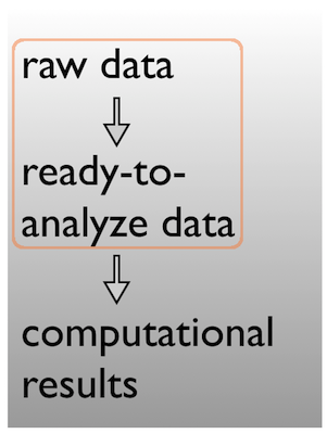\n\n~~~\ndata\ndata-raw\ndata-clean\ndata/\n - raw\n - clean\n~~~\n\n
\n\n---\n\n## Data -> results\n\nPick a strategy, any strategy, just pick one!\n\n\n\n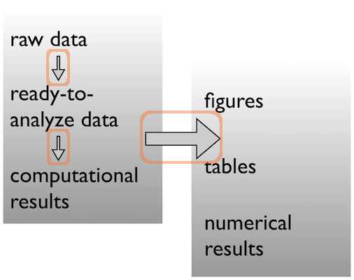\n\n~~~\ncode\nscripts\nanalysis\nbin\n~~~\n
\n\n---\n\n## Data -> results\n\nPick a strategy, any strategy, just pick one!\n\n\n\n\n\n~~~\nfigures\nresults\nresults/\n - figs\n - nums\nfigures\ntables\n~~~\n
\n\n---\n\n## A real (and imperfect!) example\n\n~~~\n /Users/jenny/research/bohlmann/White_Pine_Weevil_DE:\n total used in directory 246648 available 131544558\n drwxr-xr-x 14 jenny staff 476 Jun 23 2014 .\n drwxr-xr-x 4 jenny staff 136 Jun 23 2014 ..\n -rw-r--r--@ 1 jenny staff 15364 Apr 23 10:19 .DS_Store\n -rw-r--r-- 1 jenny staff 126231190 Jun 23 2014 .RData\n -rw-r--r-- 1 jenny staff 19148 Jun 23 2014 .Rhistory\n drwxr-xr-x 3 jenny staff 102 May 16 2014 .Rproj.user\n drwxr-xr-x 17 jenny staff 578 Apr 29 10:20 .git\n -rw-r--r-- 1 jenny staff 50 May 30 2014 .gitignore\n -rw-r--r-- 1 jenny staff 1003 Jun 23 2014 README.md\n -rw-r--r-- 1 jenny staff 205 Jun 3 2014 White_Pine_Weevil_DE.Rproj\n drwxr-xr-x 20 jenny staff 680 Apr 14 15:44 analysis\n drwxr-xr-x 7 jenny staff 238 Jun 3 2014 data\n drwxr-xr-x 22 jenny staff 748 Jun 23 2014 model-exposition\n drwxr-xr-x 4 jenny staff 136 Jun 3 2014 results\n~~~\n\n---\n\n## Data\n\nReady to analyze data:\n\n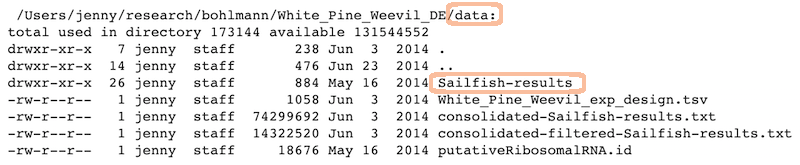\n\n
\n\nRaw data:\n\n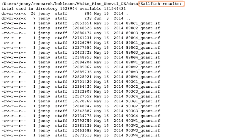\n\n\n---\n\n## Analysis and figures\n\nR scripts + the Markdown files from \"Compile Notebook\":\n\n\n\n
\n\nThe figures created in those R scripts and linked in those Markdown files:\n\n\n\n## Scripts\n\nLinear progression of R scripts, and Makefile to run the entire analysis:\n\n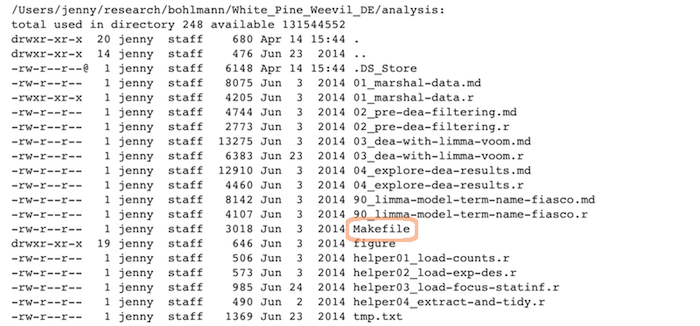\n\n## Results\n\nTab-delimited files with one row per gene of parameter estimates, test statistics, etc.:\n\n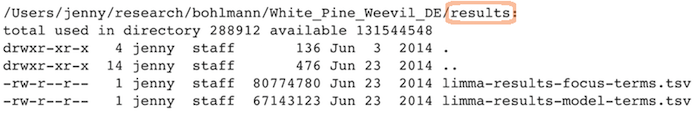\n\n## Expository files\n\nFiles to help collaborators understand the model we fit: some markdown docs, a Keynote presentation, Keynote slides exported as PNGs for viewability on GitHub:\n\n\n\n---\n\n## Caveats / problems with this example\n\n- This project is no where near done, i.e. no manuscript or publication-ready figs\n\n- File naming has inconsistencies due to three different people being involved\n\n- Code and reports/figures all sit together because it’s just much easier that way w/ knitr & rmarkdown\n\n---\n\n## Wins of this example\n\n- I can walk away from the project and come back to it a year later and resume work fairly quickly\n\n- The two other people were able to figure out what I did and decide which files they needed to look at, etc.\n\n---\n\n## Tip: Life cycle of data\n\nHere’s how most data analyses go down in reality:\n\n- You get raw data\n\n- You explore, describe and visualize it\n\n- You diagnose what this data needs to become useful\n\n- You fix, clean, marshal the data into ready-to-analyze form\n\n- You visualize it some more\n\n- You fit a model or whatever and write lots of numerical results to file\n\n- You make prettier tables and many figures based on the data & results accumulated by this point\n\nBoth the data file(s) and the code/scripts that acts on them reflect this progression\n\n---\n\n## Prepare data -> Do stats -> Make tables & figs\n\nThe R scripts:\n\n~~~\n01_marshal-data.r\n02_pre-dea-filtering.r\n03_dea-with-limma-voom.r\n~~~\n\n
\n\nThe figures left behind:\n\n~~~\n02_pre-dea-filtering-preDE-filtering.png\n03-dea-with-limma-voom-voom-plot.png\n04_explore-dea-results-focus-term-adjusted-p-values1.png\n04_explore-dea-results-focus-term-adjusted-p-values2.png\n~~~\n\nFile organization should reflect inputs vs outputs and the flow of information\n\nSource [Data Carpentry](https://datacarpentry.org/rr-organization1/02-file-organization/index.html)\n---\n\n# Let's Practice!","fields":{"slug":"/chapter7_02_project_organization"}}},{"node":{"rawMarkdownBody":"\n Lesson 4
Testing
Lesson 8
Software Licensing
Lesson 7
Introduction to CI/CD and Github Actions
 \n\n\n---\n\n3. Click on the first “Simple workflow” configure button\n\n\n
 \n\n\n---\n\n4. Click on the two green commit buttons to add this workflow file\n\n\n
 \n\n---\n\n5. Go back to the “Actions” tab. It now looks different:\n\n\n
 \n\n\n---\n\n6. Click on the message associated with the event that created the action:\n\n\n
 \n\n---\n\n7. Click on the build link:\n\n\n
 \n\n---\n\n8. Click on the arrow inside the build logs to expand a section and see the output of the action Check all of the arrows and see what happens at each step.\n\n\n
 \n\n---\n\n## GitHub Actions workflow file\n\nA YAML file that lives in the .github/workflows directory or your repository which speciies your workflow.\n\nA basic example of this yaml file:\n\n```\nname: learn-github-actions\non: [push]\njobs:\n check-bats-version:\n runs-on: ubuntu-latest\n steps:\n - uses: actions/checkout@v2\n - uses: actions/setup-node@v2\n with:\n node-version: '14'\n - run: npm install -g bats\n - run: bats -v\n```\n\n---\n\n## Understanding the file\n\n| | |\n| ----------------- | -----------------------------|\n| name: learn-github-actions | Optional - The name of the workflow as it will appear in the Actions tab of the GitHub repository. |\n| on: [push] | Specifies the trigger for this workflow. This example uses the push event, so a workflow run is triggered every time someone pushes a change to the repository |\n| jobs: | Groups together all the jobs that run in the learn-github-actions workflow. |\n| check-bats-version: | Defines a job named check-bats-version. The child keys will define properties of the job. |\n| runs-on: ubuntu-latest | Configures the job to run on the latest version of an Ubuntu Linux runner. This means that the job will execute on a fresh virtual machine hosted by GitHub. |\n| steps: | Groups all the steps that run in the check-bats-version job. |\n| uses: actions/checkout@v2 | The uses keyword specifies that this step will run v2 of the actions/checkout action. |\n| uses: actions/setup-node@v2 with: node-version: '14' | This step uses the actions/setup-node@v2 action to install the specified version of the Node.js (this example uses v14). This puts both the node and npm commands in your PATH. |\n| run: npm install -g bats | The run keyword tells the job to execute a command on the runner. |\n| run: bats -v | Run the bats command with a parameter that outputs the software version. |\n\n\n---\n# Let's practice what we learned!\n","fields":{"slug":"/chapter7_05_github_actions"}}},{"node":{"rawMarkdownBody":"\n
 Lesson 3
Data Workflows